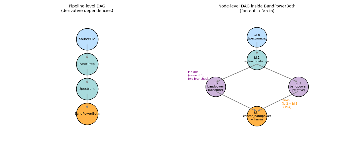
DAG Capabilities: Branching and Multi-Input Nodes

This example demonstrates the core DAG structural patterns in NeuroDAGs:

1. Linear chain — nodes executing sequentially (BasicPrep → Spectrum)

2. Fan-out — one node’s output feeds two independent branches

3. Fan-in — a single node that depends on two previous nodes

4. YAML configuration — pipeline defined as a readable YAML string

5. Custom inline nodes — register your own node without a separate file

Pipeline graph:

  SourceFile
      │
  BasicPrep  (linear chain)
      │
  Spectrum
      │
  id.1: extract_data_var
     ╱ ╲
id.2   id.3          ← fan-out: same upstream, two parallel branches
(abs)   (rel)
   ╲ ╱
  id.4: concat_bandpower  ← fan-in: depends on BOTH id.2 and id.3

Setup

import tempfile
from pathlib import Path

import matplotlib

matplotlib.use("Agg")
import matplotlib.pyplot as plt
import numpy as np
import xarray as xr
import yaml

from neurodags.datasets import generate_dummy_dataset
from neurodags.definitions import Artifact, NodeResult
from neurodags.nodes import register_node
from neurodags.orchestrators import build_derivative_dataframe, run_pipeline

WORKDIR = Path(tempfile.mkdtemp(prefix="neurodags_dag_"))
DATA_DIR = WORKDIR / "rawdata"
OUT_DIR = WORKDIR / "derivatives"
OUT_DIR.mkdir(parents=True, exist_ok=True)

print(f"Working directory: {WORKDIR}")

Working directory: /tmp/neurodags_dag_wmkcuyqm

Custom node — the fan-in (two-input) example

Register a node that accepts two upstream DataArrays and concatenates them along a new normalization coordinate.

This is the key pattern: one node, two predecessor branches.

@register_node(name="concat_bandpower", override=True)
def concat_bandpower(absolute, relative) -> NodeResult:
    """Stack absolute and relative band power along a new 'normalization' axis."""
    if isinstance(absolute, NodeResult):
        absolute = absolute.artifacts[".nc"].item
    if isinstance(relative, NodeResult):
        relative = relative.artifacts[".nc"].item
    combined = xr.concat(
        [absolute, relative],
        dim=xr.DataArray(["absolute", "relative"], dims="normalization"),
    )
    combined.name = "bandpower"
    return NodeResult(
        artifacts={".nc": Artifact(item=combined, writer=lambda p: combined.to_netcdf(p))}
    )

Step 1 — Generate Synthetic Dataset

Two subjects, 10 seconds each — enough for a branching-pipeline demo.

generate_dummy_dataset(
    data_params={
        "DATASET": "dag_demo",
        "PATTERN": "sub-%subject%/sub-%subject%_task-rest",
        "NSUBS": 2,
        "NSESSIONS": 1,
        "NTASKS": 1,
        "NACQS": 1,
        "NRUNS": 1,
        "PREFIXES": {
            "subject": "S",
            "session": "SE",
            "task": "T",
            "acquisition": "A",
            "run": "R",
        },
        "ROOT": str(DATA_DIR),
    },
    generation_args={
        "NCHANNELS": 8,
        "SFREQ": 200.0,
        "STOP": 10.0,
        "NUMEVENTS": 5,
        "random_state": 0,
    },
)

source_files = sorted(DATA_DIR.rglob("*.vhdr"))
print(f"Generated {len(source_files)} source file(s)")

Creating RawArray with float64 data, n_channels=8, n_times=2000
    Range : 0 ... 1999 =      0.000 ...     9.995 secs
Ready.
/home/runner/work/neurodags/neurodags/src/neurodags/datasets.py:703: RuntimeWarning: Encountered data in 'double' format. Converting to float32.
  export_raw(fname=str(vhdr_path), raw=raw, fmt="brainvision", overwrite=True)
Generated 2 source file(s)

Step 2 — Datasets config as YAML

Defining datasets in YAML keeps the configuration version-controlled and separate from code. For reproducible workflows, save this string to a .yml file and point load_configuration at it.

DATASETS_YAML = f"""\
dag_demo:
  name: DAG Demo
  file_pattern: "{DATA_DIR / '**' / '*.vhdr'}"
  derivatives_path: "{OUT_DIR}"
"""

datasets = yaml.safe_load(DATASETS_YAML)
print("Datasets:", list(datasets))

Datasets: ['dag_demo']

Step 3 — Pipeline config as YAML

The BandPowerBoth derivative shows all three DAG patterns:

• id.0 loads the cached Spectrum artifact (cross-derivative dependency)

• id.1 extracts the spectrum array (linear step)

• id.2 and id.3 both read from id.1 → fan-out

• id.4 reads from both id.2 and id.3 → fan-in

PIPELINE_YAML = """\
mount_point: null

DerivativeDefinitions:

  # ── 1. Linear chain ─────────────────────────────────────────────────────
  BasicPrep:
    overwrite: false
    nodes:
      - id: 0
        derivative: SourceFile
      - id: 1
        node: basic_preprocessing
        args:
          mne_object: id.0
          filter_args: {l_freq: 1.0, h_freq: 80.0}
          epoch_config: {duration: 2.0, overlap: 0.0}

  Spectrum:
    overwrite: false
    nodes:
      - id: 0
        derivative: BasicPrep.fif
      - id: 1
        node: mne_spectrum_array
        args:
          meeg: id.0
          method: welch
          method_kwargs: {n_per_seg: 200}

  # ── 2. Fan-out then fan-in ───────────────────────────────────────────────
  BandPowerBoth:
    save: false        # computed on-the-fly; not written to disk
    for_dataframe: true
    nodes:
      - id: 0
        derivative: Spectrum.nc   # load cached cross-derivative result

      - id: 1            # shared upstream for both branches
        node: extract_data_var
        args: {dataset_like: id.0, data_var: spectrum}

      - id: 2            # branch A — absolute power (fan-out from id.1)
        node: bandpower
        args:
          psd_like: id.1
          relative: false
          bands:
            delta: [1.0,  4.0]
            alpha: [8.0, 13.0]
            beta:  [13.0, 30.0]

      - id: 3            # branch B — relative power (fan-out from id.1)
        node: bandpower
        args:
          psd_like: id.1
          relative: true
          bands:
            delta: [1.0,  4.0]
            alpha: [8.0, 13.0]
            beta:  [13.0, 30.0]

      - id: 4            # fan-in: depends on BOTH id.2 (abs) and id.3 (rel)
        node: concat_bandpower
        args:
          absolute: id.2
          relative: id.3

DerivativeList:
  - BasicPrep
  - Spectrum
  - BandPowerBoth
"""

pipeline_config = yaml.safe_load(PIPELINE_YAML)
pipeline_config["datasets"] = datasets

print("Pipeline derivatives:", pipeline_config["DerivativeList"])

Pipeline derivatives: ['BasicPrep', 'Spectrum', 'BandPowerBoth']

Step 4 — Visualise the DAG structure

Draw the node-level graph for BandPowerBoth before executing anything.

fig, axes = plt.subplots(1, 2, figsize=(12, 5))

# Left: cross-derivative pipeline DAG
ax = axes[0]
deriv_positions = {
    "SourceFile": (2, 4),
    "BasicPrep": (2, 3),
    "Spectrum": (2, 2),
    "BandPowerBoth": (2, 1),
}
deriv_colors = {
    "SourceFile": "#bde0fe",
    "BasicPrep": "#a8dadc",
    "Spectrum": "#a8dadc",
    "BandPowerBoth": "#ffb347",
}
for name, (x, y) in deriv_positions.items():
    ax.scatter(x, y, s=3000, c=deriv_colors[name], zorder=3, edgecolors="black", linewidths=1.2)
    ax.text(x, y, name, ha="center", va="center", fontsize=8, zorder=4)

for src, dst in [
    ("SourceFile", "BasicPrep"),
    ("BasicPrep", "Spectrum"),
    ("Spectrum", "BandPowerBoth"),
]:
    x0, y0 = deriv_positions[src]
    x1, y1 = deriv_positions[dst]
    ax.annotate(
        "",
        xy=(x1, y1 + 0.18),
        xytext=(x0, y0 - 0.18),
        arrowprops={"arrowstyle": "->", "color": "gray", "lw": 1.5},
    )

ax.set_xlim(0, 4)
ax.set_ylim(0, 5)
ax.axis("off")
ax.set_title("Pipeline-level DAG\n(derivative dependencies)", fontsize=10)

# Right: node-level DAG inside BandPowerBoth
ax = axes[1]
node_positions = {
    0: (3, 4.5),
    1: (3, 3.5),
    2: (1.5, 2.3),
    3: (4.5, 2.3),
    4: (3, 1),
}
node_labels = {
    0: "id.0\nSpectrum.nc",
    1: "id.1\nextract_data_var",
    2: "id.2\nbandpower\n(absolute)",
    3: "id.3\nbandpower\n(relative)",
    4: "id.4\nconcat_bandpower\n← fan-in",
}
node_colors = {0: "#bde0fe", 1: "#a8dadc", 2: "#cdb4db", 3: "#cdb4db", 4: "#ffb347"}
node_edges = [(0, 1), (1, 2), (1, 3), (2, 4), (3, 4)]

for nid, (x, y) in node_positions.items():
    ax.scatter(x, y, s=2500, c=node_colors[nid], zorder=3, edgecolors="black", linewidths=1.2)
    ax.text(x, y, node_labels[nid], ha="center", va="center", fontsize=7.5, zorder=4)

for src, dst in node_edges:
    x0, y0 = node_positions[src]
    x1, y1 = node_positions[dst]
    ax.annotate(
        "",
        xy=(x1, y1 + 0.2),
        xytext=(x0, y0 - 0.2),
        arrowprops={"arrowstyle": "->", "color": "gray", "lw": 1.5},
    )

# annotate the fan-out and fan-in
ax.text(0.5, 2.8, "fan-out\n(same id.1,\ntwo branches)", fontsize=7, color="purple", va="center")
ax.text(3.9, 1.55, "fan-in\n(id.2 + id.3\n→ id.4)", fontsize=7, color="darkorange", va="center")

ax.set_xlim(0, 6)
ax.set_ylim(0, 5.5)
ax.axis("off")
ax.set_title("Node-level DAG inside BandPowerBoth\n(fan-out → fan-in)", fontsize=10)

plt.tight_layout()
plt.savefig(WORKDIR / "dag_structure.png", dpi=100)
plt.show()
print(f"DAG diagram saved to {WORKDIR / 'dag_structure.png'}")

DAG diagram saved to /tmp/neurodags_dag_wmkcuyqm/dag_structure.png

Step 5 — Execute the Pipeline

run_pipeline runs all derivatives in DerivativeList, sorted by dependency order. Already-cached outputs are skipped.

run_pipeline(pipeline_config, raise_on_error=True)

produced = sorted(OUT_DIR.rglob("*@*.fif")) + sorted(OUT_DIR.rglob("*@*.nc"))
print(f"\nProduced {len(produced)} derivative file(s):")
for f in produced:
    print(f"  {f.relative_to(WORKDIR)}")

Not setting metadata
5 matching events found
No baseline correction applied
0 projection items activated
Using data from preloaded Raw for 5 events and 400 original time points ...
0 bad epochs dropped
/home/runner/work/neurodags/neurodags/src/neurodags/nodes/preprocessing.py:143: RuntimeWarning: This filename (/tmp/neurodags_dag_wmkcuyqm/derivatives/sub-S1/sub-S1_task-rest.vhdr@BasicPrep.fif) does not conform to MNE naming conventions. All epochs files should end with -epo.fif, -epo.fif.gz, _epo.fif or _epo.fif.gz
  ".fif": Artifact(item=mne_object, writer=lambda path: mne_object.save(path, overwrite=True))
Not setting metadata
5 matching events found
No baseline correction applied
0 projection items activated
Using data from preloaded Raw for 5 events and 400 original time points ...
0 bad epochs dropped
/home/runner/work/neurodags/neurodags/src/neurodags/nodes/preprocessing.py:143: RuntimeWarning: This filename (/tmp/neurodags_dag_wmkcuyqm/derivatives/sub-S0/sub-S0_task-rest.vhdr@BasicPrep.fif) does not conform to MNE naming conventions. All epochs files should end with -epo.fif, -epo.fif.gz, _epo.fif or _epo.fif.gz
  ".fif": Artifact(item=mne_object, writer=lambda path: mne_object.save(path, overwrite=True))
Effective window size : 1.280 (s)
Effective window size : 1.280 (s)

Produced 4 derivative file(s):
  derivatives/sub-S0/sub-S0_task-rest.vhdr@BasicPrep.fif
  derivatives/sub-S1/sub-S1_task-rest.vhdr@BasicPrep.fif
  derivatives/sub-S0/sub-S0_task-rest.vhdr@Spectrum.nc
  derivatives/sub-S1/sub-S1_task-rest.vhdr@Spectrum.nc

Step 6 — Inspect the Fan-in Result

build_derivative_dataframe collects for_dataframe=True derivatives. BandPowerBoth re-runs the full node chain (id.0–id.4) and flattens the 4-D result (epochs × channels × freqbands × normalization) into columns.

df = build_derivative_dataframe(pipeline_config, output_format="wide")
df["subject"] = df["file_path"].apply(
    lambda p: next(
        (part for part in Path(p).parts if part.startswith("sub-")),
        Path(p).stem,
    )
)
print(f"DataFrame shape: {df.shape}")
band_cols = [c for c in df.columns if "BandPower" in c]
print(f"Band-power columns ({len(band_cols)}):", band_cols[:6], "...")

DataFrame shape: (2, 244)
Band-power columns (240): ['BandPowerBoth.nc@epochs-0_freqbands-delta_normalization-absolute_spaces-EEG000', 'BandPowerBoth.nc@epochs-0_freqbands-alpha_normalization-absolute_spaces-EEG000', 'BandPowerBoth.nc@epochs-0_freqbands-beta_normalization-absolute_spaces-EEG000', 'BandPowerBoth.nc@epochs-0_freqbands-delta_normalization-absolute_spaces-EEG001', 'BandPowerBoth.nc@epochs-0_freqbands-alpha_normalization-absolute_spaces-EEG001', 'BandPowerBoth.nc@epochs-0_freqbands-beta_normalization-absolute_spaces-EEG001'] ...

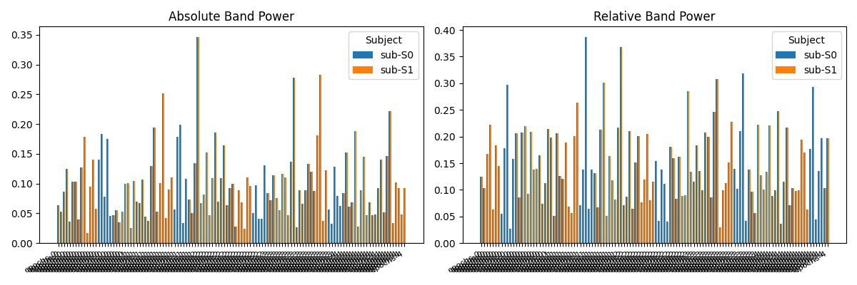
Step 7 — Plot Band Power by Normalization Type

Separate the absolute and relative columns and compare them side-by-side.

abs_cols = [c for c in band_cols if "absolute" in c]
rel_cols = [c for c in band_cols if "relative" in c]

if abs_cols and rel_cols:
    subjects = sorted(df["subject"].unique())
    n_subs = len(subjects)
    x = np.arange(len(abs_cols))
    width = 0.8 / n_subs

    fig, axes = plt.subplots(1, 2, figsize=(12, 4), sharey=False)

    for ax, cols, title in zip(
        axes,
        [abs_cols, rel_cols],
        ["Absolute Band Power", "Relative Band Power"],
        strict=False,
    ):
        for i, sub in enumerate(subjects):
            row = df[df["subject"] == sub]
            vals = row[cols].mean(axis=0).values if not row.empty else np.zeros(len(cols))
            ax.bar(x + i * width, vals, width=width, label=sub)
        ax.set_xticks(x + width * (n_subs - 1) / 2)
        short_labels = [c.split("@")[-1].split("_")[0] for c in cols]
        ax.set_xticklabels(short_labels, rotation=30, ha="right", fontsize=8)
        ax.set_title(title)
        ax.legend(title="Subject")

    plt.tight_layout()
    plt.savefig(WORKDIR / "band_power_both.png", dpi=100)
    plt.show()
    print(f"Plot saved to {WORKDIR / 'band_power_both.png'}")
else:
    print("No band-power columns found — check pipeline execution.")

Plot saved to /tmp/neurodags_dag_wmkcuyqm/band_power_both.png

Summary

Key takeaways:

• YAML config makes pipelines readable and version-controllable.

• The same pipeline can be driven from the CLI with neurodags validate, neurodags run, neurodags dry-run, neurodags dataframe, and neurodags dag.

• Custom nodes (@register_node) integrate seamlessly — no plugins needed.

• Fan-out: point multiple node args at the same id.N.

• Fan-in: list multiple id.N references in one node’s args; the topological sorter resolves execution order automatically.

• The same patterns compose: chains, branches, and merges can be nested arbitrarily deep within a single derivative or across derivatives.